Predicting Peace

I have long struggled with predicting when peace will occur. Actually, I’m struggling with predicting anything relating to war1 From a list of past forecasts I had trouble with, I can find questions about territorial control changes during war, extensions of ceasefires, new entrants in conflicts, safe corridor deals, assassinations, renewal of peacekeeping missions, and arms sales., but let’s focus on when peace arrives for now. There are two such questions in the current acx 2026 competition:
- Will there be a cease-fire in Ukraine in 2026?
- Will there be a cease-fire in Sudan in 2026?
When I entered my forecast for these questions, I did it based on Laplace’s rule of succession, i.e. as a function of their duration only. This is sort of justified if war durations are heavy-tailed, which would mean that the longer they go on for, the less likely it is that peace comes soon. But I don’t know if that is true.
Either way, this first, roughest forecast is
| Question | Naïve |
|---|---|
| Ukraine | 38 % |
| Sudan | 43 % |
We’ll see if we can improve on that.
Finding data
The Uppsala Conflict Data Programme (ucdp) provides free, high-quality data on the durations of armed conflicts. This is their extensive conflict termination dataset covering all armed conflicts (interstate and intrastate) where there have been flare-ups of violence (called episodes in the data) after the second world war.
The following plot is a survival curve of the duration of conflict episodes started in the pc age2 It is often convenient to limit analysis to “very recent history”. I define that as the launch of the first ibm pc in 1981. It also happens to coincide with the eradiction of smallpox in 1980, meaning we can split history into the smallpox age and the pc age.. The crosses represent those that are still ongoing.
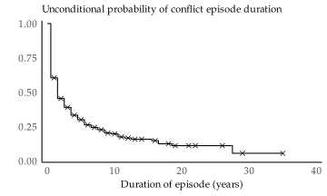
For predicting the probability of peace in the near future, we need the hazard rate. Extracting that from this data is conceptually simple – it’s the same idea as when we discussed the Supreme Court – but it turned out to be algorithmically tricky, for two reasons:
- The conflict episode data is quantised to the nearest next year. If an episode ends 3.2 years in, it will be reported in the data as having gone on for 4 years.
- A large number of episodes end early. Almost a third end after the first year, then almost a fifth in the second year.
These two properties in combination make for a weird shape of the distribution in the area around 0–2 years: conflicts that ended after 0.2 years and conflicts that ended after 0.9 years are both reported as having ended after exactly one year. The strange steppy shape of the distribution throws a typical maximum likelihood fit for a loop. After much trying of various ways of dealing with it, I figured out how to do it properly.
This gives us a theoretical distribution that fits the data well. The duration \(t\) of violent episodes is distributed as roughly
\[t \sim{} \mathrm{Weibull}(\lambda=3.4,\, k=0.5)\]
We can superimpose this on the survival function from before to get a visual confirmation of the fit. Keep in mind that we’re not saying the duration of an episode is literally determined by the Weibull distribution, only that the curve of the Weibull distribution happens to lie very close to the actual durations, so we can use the Weibull curve as an approximation of the underlying process, whatever it is.
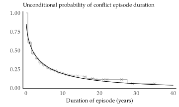
The Weibull distribution has two parameters: the scale \(\lambda\), and the shape \(k\). The interpretation of the shape parameter \(k\) is quite easy:
- \(k=1\) means the hazard rate is constant, which implies an exponential survival distribution: at any given time, a fixed percentage of the population experiences the event of interest. (In this case, that would be the end of the conflict episode.)
- \(k>1\) means the hazard rate is increasing, which implies a survival distribution that is calm at first but then quickly drops off. There is a specific region of ages at which the event of interest happens.
- \(k<1\) means the hazard rate is decreasing, which implies a survival distribution where the majority of the population experiences the event early, and then some go on for a very long time without experiencing the event.
For episode durations, we have \(k = 0.5 < 1\), which means most episodes end early, but then some go on for a very long time. If we hold \(k\) fixed at 0.5, we also get a natural interpretation of the scale parameter \(\lambda\): the average duration of a episode is \(2\lambda\). Thus, the average duration of a conflict episode in the pc age is 7 years. This might seem surprising, because the average observed episode duration in the ucdp data is something like 3.8 years! But that’s because many of those conflicts have not yet terminated, so the observed duration is biased downward.
There’s another way this is surprising: the majority of conflicts end within two years, so how can the average length be seven years? That’s thanks to the heavy-tailed nature of conflict lengths. There are a few that go on for a very long time and pull up the average length by a fair bit.
Refined estimation
Now we can actually compute a data-informed forecast of any specific ongoing conflict episode ending in the next year: it’s 11 %. We get that by taking the weighted average of the hazard rate for all durations of conflict, with weights coming from the fraction of ongoing conflicts that have been going on for that duration.
We will call this the agnostic forecast because it doesn’t care about which specific conflict we are discussing at all.
| Question | Naïve | Agnostic | Change |
|---|---|---|---|
| Ukraine | 38 % | 11 % | −1.6 log-odds |
| Sudan | 43 % | 11 % | −1.8 log-odds |
One problem with this is that the forecasting questions need a 30-day cease-fire to resolve positively, while the ucdp data counts an episode as having ended only when a full year goes by with fewer than 25 combat deaths. We should probably adjust our final forecast upwards slightly to account for that difference.
But even so, this doesn’t look like a great forecast. We’ll see where the 11 % comes from.
Duration-dependence
As we reasoned early on, and witnessed in the survival curve, the probability of peace next year depends on how long the conflict has been going on. We can use the fitted survival distribution to generate a kind of population structure of ongoing conflict episodes, i.e. the fraction of ongoing episodes we expect at each duration. Then we also extract the probability of peace in the next year from the hazard function implied by the survival distribution.
This is where agnostic 11 % came from: if we average the peace probabilities with weights taken from the fraction at each duration, we arrive at 11 %. But we can also use it to make a forecast when we know how long a conflict episode has been going on for. Instead of taking a weighted average, we read the peace probability off of the right column directly.
| Duration | Fraction | Peace probability |
|---|---|---|
| 1 year | 11 % | 27 % |
| 2 years | 8 % | 18 % |
| 3 years | 6 % | 15 % |
| 4 years | 5 % | 13 % |
| 5 years | 5 % | 12 % |
| 5–10 years | 17 % | 10 % |
| 10–20 years | 19 % | 7 % |
| 20–40 years | 16 % | 5 % |
| >40 years | 14 % | 3 % |
This table is strange in two ways. First, it might seem odd that the majority of violent episodes (66 % of them, to be precise) are older than five years, when the majority of them end within two years. This happens because we have conditioned on episodes that are ongoing, and when time-to-peace is heavy-tailed, that ends up filtering for long-running episodes.
Another thing that’s strange about this table is that the peace probabilities do not add up to unity. That’s because they are conditional probabilities, so they don’t have to. They bear no relation to each other – they apply only to episodes of the duration they are attached to.
To refine our forecast further: the Ukraine conflict has been going on for four years, and the Sudan conflict for just under three years. We pull probabilities from the table and update.
| Question | Agnostic | By duration | Change |
|---|---|---|---|
| Ukraine | 11 % | 13 % | +0.19 log-odds |
| Sudan | 11 % | 15 % | +0.36 log-odds |
That’s better, maybe, but we are probably still leaving accuracy on the table.
Accounting for types of war
We have more information we can use. The Sudan conflict is a civil war, whereas the Ukraine conflict is a war between two states. That could have a large effect on the probability of peace; when I read the news, it seems like civil wars are more difficult to stop.
Of the 411 conflict episodes in the pc age, there are only 33 interstate wars. But we can still split the data up into two categories and fit the survival distribution with civil war as a predictor.
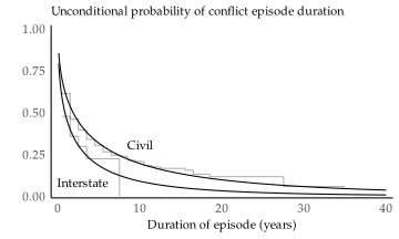
This confirms our intuition that civil wars last longer. It might even be the case that interstate wars have a completely different type of hazard rate than civil wars, but we’ll treat them the same for now.
The theoretical Weibull distribution we fitted to the data has the same shape as before (\(k\) = 0.5), but the scale now depends on whether it’s an interstate war or a civil war.
| Interstate war | Civil war |
|---|---|
| \(\lambda\) = 1.3 | \(\lambda\) = 3.6 |
As it happens, most of the average length of episodes in the data is driven by civil wars. The mean length of an interstate war in the pc age is 2.5 years, whereas for a civil war it is over 7 years. Updating our duration-agnostic forecast split up into conflict type, we have
| Interstate war | Civil war |
|---|---|
| 22 % | 10 % |
As we have seen, the peace probability depends a lot on conflict duration, so these duration-agnostic forecasts aren’t great, but they are a good way to interpret the scale of the Weibull distribution: a randomly selected interstate war is more than twice as likely to end in the next year as a civil war.
The refined table of peace probabilities conditional on duration is more useful for forecasting.
| Duration | Interstate war | Civil war |
|---|---|---|
| 1 year | 39 % | 26 % |
| 2 years | 27 % | 17 % |
| 3 years | 23 % | 14 % |
| 4 years | 20 % | 12 % |
| 5 years | 18 % | 11 % |
| 5–10 years | 15 % | 9 % |
| 10–20 years | 11 % | 7 % |
| 20–40 years | 8 % | 5 % |
| >40 years | 6 % | 3 % |
Now we get an even more accurate forecast of peace in the two wars we opened the article with.
| Question | By duration | By type | Change |
|---|---|---|---|
| Ukraine | 13 % | 20 % | +0.51 log-odds |
| Sudan | 15 % | 14 % | −0.08 log-odds |
For the first time, we have a forecast that is lower for Sudan than Ukraine. That’s because this is the first time we have accounted for it being a civil war, and civil wars generally last longer.
The point of contention
We can look into what other variables are available in the ucdp data. For example, whether the conflict is about territory or governmental control might affect how long an episode lasts. The comparison gets a little more clumsy, but here we can see the effect of whether the fight is over territory or over government.
| Fighting over… | Territory | Government |
|---|---|---|
| Interstate war | \(\lambda\) = 1.2 (n=26) | \(\lambda\) = 1.9 (n=7) |
| Civil war | \(\lambda\) = 2.9 (n=212) | \(\lambda\) = 4.8 (n=166) |
Although I would not have guessed the above results before I saw them, I think I can explain them: conflicts over who controls the population take longer to resolve than territorial disputes, because humans are more stubborn over their freedoms and ways of life than their land. Again, to aid interpretability, we can translate these scale parameters to probabilities of peace for each category.
| Fighting over… | Territory | Government |
|---|---|---|
| Interstate war | 23 % | 16 % |
| Civil war | 12 % | 8 % |
We still have that a randomly selected interstate wars is twice as likely to end than a randomly selected civil war, but now we have the added effect that a war over territory is around 1.5× as likely to end as a war over governmental control.
Although it is getting very messy, this can be broken up into duration-dependent probabilities too.
| Duration | I–T | I–G | C–T | C–G |
|---|---|---|---|---|
| 1 year | 41 % | 34 % | 28 % | 23 % |
| 2 years | 28 % | 23 % | 19 % | 15 % |
| 3 years | 23 % | 19 % | 16 % | 12 % |
| 4 years | 21 % | 17 % | 14 % | 11 % |
| 5 years | 19 % | 15 % | 12 % | 10 % |
| 5–10 years | 15 % | 12 % | 10 % | 8 % |
| 10–20 years | 11 % | 9 % | 7 % | 6 % |
| 20–40 years | 8 % | 7 % | 5 % | 4 % |
| >40 years | 6 % | 5 % | 4 % | 3 % |
We can use this to update our forecasts for the conflicts in Ukraine and Sudan. The first is an interstate war over territory, the second a civil war over government.
| Question | By type | By contention | Change |
|---|---|---|---|
| Ukraine | 20 % | 21 % | +0.06 log-odds |
| Sudan | 14 % | 12 % | −0.18 log-odds |
This latest adjustment has been smaller than the earlier ones, which makes sense. At some point, we reach the limits of the uncertainty inherent to the problem, and suffer sharply diminished returns from more information. By accounting for the main predictors – type of war and its current duration – we have probably used most of the information there is already.
But we’ll see if there’s anything else we can milk out of the dataset.
Accounting for conflict intensity
In the conflict episode termination dataset, the ucdp have coded intensity as a binary variable: low intensity is 25–1000 annual battle deaths, and more than that counts as a full-scale war. This is a dichotomisation, meaning it throws a third of the data in the rubbish bin. Fortunately, the ucdp publishes separate data sets for battle deaths, and both data sets are indexed by conflict id and year, meaning we can inner join them to get a complete data set of both durations and battle deaths.
We cannot include the raw sum of battle deaths as a predictor, because then it would leak the duration of the conflict. What we can do is count the average number of yearly battle deaths as the intensity of the conflict, and include that as a predictor. However, the distribution of battle deaths is extremely heavy-tailed.
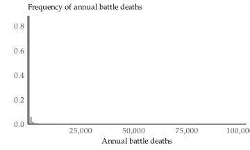
This chart goes out so far to the right because there are data points there.
Almost all conflicts have a high battle death rate; the median is nearly 100 deaths per year. Yet there are a handful of conflicts that are staggeringly violent at more than 10,000 battle deaths per year. The worst one has over 100,000 battle deaths per year. This handful of really deadly conflicts in the pc age are
- Ethiopian Tigray war (2020–2022): 103,000 battle deaths/year.
- Russia–Ukraine (2022–): 80,800 battle deaths/year.
- Ethiopia–Eritrea (1998–2000): 32,700 battle deaths/year.
- Syrian civil war (2011–2024): 20,500 battle deaths/year.
- Israel–Palestine (2018–ongoing): 12,200 battle deaths/year.
This is insanity.
32,000 battle deaths per year is almost 100 people dying every day. And that’s just among combatants, not counting civilians. I don’t even want to look up civilian casualties.
What is going on in the world?
Deep breaths.
I sometimes have to remind myself why I do this. The examples in this article are gruesome, but my hope is that (a) people realise that these things really happen in real life, and (b) at least one reader will make the world a better place using the tools I share.
If we take the logarithm of the battle death rate we get a more tractable distribution.
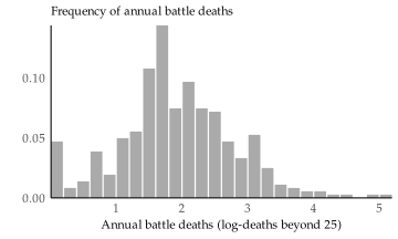
Here we have taken the logarithm base ten, so that the number indicates how many zeroes there are in the number. For example, 4 should be read as 10,000. From this plot, it is clear that the median is somewhere around 100 annual battle deaths. The standard deviation is nearly an order of magnitude.
When we include this variable in the model, the variable that indicated whether the fight was over territory or government drops out. It seems that it mostly served as a proxy for the level of violence in the conflict. The shape \(k\) goes up to 0.7, and to get the scale, we need an estimation of the order of magnitude of the intensity.
| Log-intensity | 1 | 2 | 3 | 4 | 5 |
|---|---|---|---|---|---|
| Interstate war | \(\lambda\) = 0.4 | 1.7 | 8.7 | 43 | 214 |
| Civil war | \(\lambda\) = 0.8 | 3.7 | 19 | 92 | 460 |
For interpretability reasons, we can convert this to a probability of peace when ignorant of their duration
| Log-intensity | 1 | 2 | 3 | 4 | 5 |
|---|---|---|---|---|---|
| Interstate war | 74 % | 32 % | 8 % | 2 % | <1 % |
| Civil war | 52 % | 17 % | 4 % | 1 % | <1 % |
This would indicate probabilities of <1 % for the Ukraine conflict (interstate ware with annual battle death rate \(10^5\)), and 4 % for the Sudan conflict (civil war with annual battle death rate \(10^3\)). However, we also need to account for their duration.
First, for interstate wars:
| Log-intensity | 1 | 2 | 3 | 4 | 5 |
|---|---|---|---|---|---|
| 1 year | 77 % | 40 % | 15 % | 5 % | 2 % |
| 2 years | 67 % | 33 % | 12 % | 4 % | 1 % |
| 3 years | 62 % | 30 % | 11 % | 4 % | 1 % |
| 4 years | 59 % | 27 % | 10 % | 3 % | 1 % |
| 5 years | 56 % | 26 % | 9 % | 3 % | 1 % |
| 5–10 years | 53 % | 23 % | 8 % | 3 % | <1 % |
| 10–20 years | 47 % | 20 % | 7 % | 2 % | <1 % |
| 20–40 years | 41 % | 17 % | 6 % | 2 % | <1 % |
| >40 years | 33 % | 14 % | 4 % | 1 % | <1 % |
and then for civil wars:
| Log-intensity | 1 | 2 | 3 | 4 | 5 |
|---|---|---|---|---|---|
| 1 year | 59 % | 26 % | 9 % | 3 % | 1 % |
| 2 years | 49 % | 21 % | 7 % | 2 % | <1 % |
| 3 years | 45 % | 18 % | 6 % | 2 % | <1 % |
| 4 years | 42 % | 17 % | 6 % | 2 % | <1 % |
| 5 years | 40 % | 16 % | 5 % | 2 % | <1 % |
| 5–10 years | 37 % | 14 % | 5 % | 2 % | <1 % |
| 10–20 years | 32 % | 12 % | 4 % | 1 % | <1 % |
| 20–40 years | 27 % | 10 % | 3 % | 1 % | <1 % |
| >40 years | 22 % | 8 % | 2 % | <1 % | <1 % |
Of course, we don’t actually have data to fill all these fine-grained buckets. We have made assumptions about how the data we do have are related to each other, and used that to interpolate and extrapolate to where data is missing. With this, our forecast for the two conflicts we opened with should be
| Question | By contention | By raw intensity |
|---|---|---|
| Ukraine | 21 % | 1 % |
| Sudan | 12 % | 6 % |
Well … I’m not sure what I think about that. Our model leads us to predict 1 % for every extremely high-intensity (\(10^5\)) conflict. That’s obviously the wrong prediction: those conflicts do end far sooner than in the 100 years implied by the 1 % success rate. I would personally maybe not distinguish between conflict intensities above \(10^3\), and use the probabilities for \(10^3\) conflicts for those too. We can encode that intuition into the model by breaking the intensity up into three bands:
- Low intensity: fewer than 50 annual battle deaths. (30 % of the data.)
- High intensity: more than 200 annual battle deaths. (31 % of the data.)
In between, we find the median, baseline intensity. The shape of the Weibull distribution fitted to these predictors is 0.6.
| Intensity | Low | Median | High |
|---|---|---|---|
| Interstate war | \(\lambda\) = 0.5 | 1.4 | 6.2 |
| Civil war | \(\lambda\) = 1.0 | 3.1 | 13 |
Translated to duration-agnostic probabilities of peace for interpretation:
| Intensity | Low | Median | High |
|---|---|---|---|
| Interstate war | 55 % | 29 % | 9 % |
| Civil war | 36 % | 16 % | 4 % |
The duration-dependent probabilities for interstate wars would then be
| Intensity | Low | Median | High |
|---|---|---|---|
| 1 year | 64 % | 42 % | 20 % |
| 2 years | 51 % | 32 % | 14 % |
| 3 years | 45 % | 27 % | 12 % |
| 4 years | 41 % | 25 % | 11 % |
| 5 years | 38 % | 23 % | 10 % |
| 5–10 years | 34 % | 20 % | 9 % |
| 10–20 years | 28 % | 16 % | 7 % |
| 20–40 years | 22 % | 12 % | 5 % |
| >40 years | 17 % | 10 % | 4 % |
For civil wars they are
| Intensity | Low | Median | High |
|---|---|---|---|
| 1 year | 49 % | 28 % | 13 % |
| 2 years | 37 % | 21 % | 9 % |
| 3 years | 32 % | 18 % | 8 % |
| 4 years | 29 % | 16 % | 7 % |
| 5 years | 27 % | 15 % | 7 % |
| 5–10 years | 24 % | 13 % | 6 % |
| 10–20 years | 19 % | 10 % | 4 % |
| 20–40 years | 15 % | 8 % | 3 % |
| >40 years | 12 % | 6 % | 2 % |
Converted to a forecast, we get.
| Question | By contention | By intensity |
|---|---|---|
| Ukraine | 21 % | 11 % |
| Sudan | 12 % | 8 % |
These probabilities still need to be adjusted because the resolution criteria for the forecasting competition are looser than in the ucdp data, so I would add maybe one log-odds to both probabilities, and end up with a final forecast of
| Question | By contention | Forecast | Change |
|---|---|---|---|
| Ukraine | 21 % | 25 % | +0.23 log-odds |
| Sudan | 12 % | 19 % | +0.54 log-odds |
That feels reasonable. It is lower than my naïve forecasts of 38 % and 43 % respectively, but that also reflects my main takeaway from this analysis: conflicts last much longer than I think. Since so many of them resolve so quickly, it is easy to accidentally think that those that are currently ongoing will resolve soon, too. But by looking at those that are ongoing now, we are filtering for those that are long-running, thanks to the heavy tails of the distribution of their duration.
Appendix A: estimation of conflict episode cost
Although it is of no help for answering the forecasting question we have, we can also analyse the cost of conflict episodes. We have battle death estimations of 362 of the episodes in the pc age.
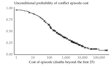
Half of conflict episodes end before 300 battle deaths. Of those that go on, half again end before 3,000 battle deaths. Of those that go on, half again end before 30,000 battle deaths. Of those that go on, we don’t yet have numbers to accurately estimate when half of them end, but it wouldn’t be weird to assume that they end before 300,000 battle deaths.
But that also means half of those continue further, even after 300,000 deaths in battle. That’s 0.3 million people whose lives are no longer. Whose family misses them. Whose children will either never be, or never see their parent again.