Nvidia Stock Crash Prediction

One of the questions of the 2026 acx prediction contest is whether Nvidia’s stock price will close below $100 on any day in 2026. At the time of writing, it trades at $184 and a bit, so going down to $100 would be a near halving of the stock value of the highest valued company in the world.
It’s an interesting question, and it’s worth spending some time on it.
If you just want the answer, my best prediction is that the probability is around 10 %. I didn’t expect to get such a high answer, but read on to see how we can find out.
When we predicted the Dow Jones index crossing a barrier in 2023, we treated the index as an unbiased random walk. That was convenient, but we cannot do it with the Nvidia question because of one major difference: the time scale.
Return grows faster than volatility
Over short time spans, the volatility1 Or noise, or variation, or standard deviation. of stock movements dominate their return2 Or signal, or drift, or average change.. This happens because noise grows with the square root of time, while signal grows linearly with time.
The plot below illustrates an imaginary amazing investment which has a yearly log-return of 0.3, and a yearly volatility of 0.3.3 Readers aware that stonks go up will recognise this as an unrealistic Sharpe ratio of 1.0. The middle line follows our best guess for how the investment will grow after each year, and the outer curves illustrate our uncertainty around the exact value of it.

Early on, we can see that the uncertainty is much bigger than the height to the trend line. Before a year has passed, the exact result is determined more by noise than by growth. Toward the end, growth has taken over and the noise has a smaller effect.
One measure of how much volatility there is compared to expected return is the signal-to-noise ratio. It’s computed as
\[10 \log_{10}\left(\frac{\mu\sqrt{t}}{\sigma}\right)\]
and for the Dow Jones question, we were looking at a signal-to-noise ratio of −8 dB. That is already a little too high to safely assume it behaves like an unbiased random walk, but for a low-stakes prediction contest it works out.
Using return data for the Nvidia stock from 2025, the signal-to-noise ratio is −1.4 dB. Although the movement in this period is still dominated by noise4 Evidenced by negative signal-to-noise ratio., the expected return is still going to matter, and we shouldn’t assume it behaves like an unbiased random walk.
Volatility is not constant over a year
Even if we ignore the problematic signal-to-noise ratio and pretend the Nvidia stock price is an unbiased random walk, we’ll run into what’s perhaps the bigger problem: the theory of unbiased random walks assumes constant volatility throughout the year. The computer will happily tell us there is a near-zero percent chance of the stock closing under $100 at any point next year.

The computer does grant a 23 % probability that the stock price drops to $130, and that might get us thinking. If we assume the stock price has dropped to $130, that tells us something about the market environment we’re in. Nvidia might drop to $130 due to random chance alone, but it’s more likely to do that if we’re in a market with a higher volatility than we assumed based on the 2025 returns. In such a market, a further drop to $100 isn’t so strange anymore.
Our simple random walk model does not account for this. When forecasting stock prices over longer periods, we need a better understanding of how the volatility might change in the future.
Options traders estimate volatility for breakfast
Fortunately for us, there are people who continuously estimate the volatility of specific stock prices. They even do it in relation to barriers like the $100 price we’re interested in. They’re options traders!
The expected volatility of the stock price is one of the variables that go into pricing an option. This means we can look up a December 2026 Nvidia call option with a strike price of $100 in the market, see what it costs, and then reverse the option pricing process to get an implied volatility out.
To do this, we first need to learn how to price an option, and to do that, we need to know what an option is.
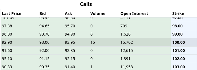
In this article, we’re going to focus on call options because they are more thickly traded. Assume we have an un-expired Nvidia call option with a strike price of $100. We can then exercise it, which means we trade in the option plus the strike price for one share in the underlying Nvidia stock. If we did that today, we would earn $84, because we lose the $100, but the share in Nvidia we get in exchange is worth $184.
We don’t have to exercise the option, though. If the price of Nvidia goes up tomorrow, we would earn more from exercising the option tomorrow. We can delay exercising it right up until it expires, when it becomes invalid.
If we were able to buy the $100 option for less than $84, we would get free profit. The chart above tells us, however, that the $100 option costs $92.90, meaning the market expects there to be a better opportunity for exercising that option before it expires.
The binomial asset price model
To keep things computationally simple, we are going to use a binomial model for the price of the underlying Nvidia stock. We don’t know the daily volatility, so we’ll keep that as a variable we call \(\sigma\). We will pretend that each day, the Nvidia stock price can either grow with a factor of \(e^\sigma\) or shrink with a factor of \(e^{-\sigma}\).5 This is a geometric binomial walk. We could transform everything in the reasoning below with the logarithm and get an additive walk in log-returns.
Thus, on day zero, the Nvidia stock trades for $184. On day one, it can take one of two values:
- \(184e^\sigma\) because it went up, or
- \(184e^{-\sigma}\) because it went down.
On day two, it can have one of three values:
- \(184e^{2\sigma}\) (went up both in the first and second day),
- \(184e^{\sigma - \sigma} = 184\) (went up and then down, or vice versa), or
- \(184e^{-2\sigma}\) (went down both days).
If it’s easier, we can visualise this as a tree. Each day, the stock price branches into two possibilities, one where it rises, and one where it goes down. In the graph below, each column of bubbles represents the closing value for a day.

This looks like a very crude approximation, but it actually works if the time steps are fine-grained enough. The uncertainties involved in some of the other estimations we’ll do dwarf the inaccuracies introduced by this model.6 Even for fairly serious use, I wouldn’t be unhappy with daily time steps when the analysis goes a year out.
It is important to keep in mind that the specific numbers in the bubbles depend on which number we selected for the daily volatility \(\sigma\). Any conclusion we draw from this tree is a function of the specific \(\sigma\) chosen to construct the tree.
When we have chosen an initial \(\sigma\) and constructed this tree, we can price an option using it. Maybe we have a call option expiring on day three, with a strike price of $180. On day four, the last day, the option has expired, so it is worth nothing. We’ll put that into the tree.

We have already seen what the value of the option is on the day it expires: it’s what we would profit from exercising it. If the stock is valued at $191, the option is worth $11, the difference between the stock value and the strike price. On the other hand, if the stock is valued at $177, it is worth less than the strike price of the option, so we will not exercise the option, instead letting it expire.

The day before the expiration day is when we have the first interesting choice to make. We can still exercise the option, with the exercise value of the option calculated the same way.
Or we could hold on to the option. If we hold on to the option for a day, the value of the option will either go up or down, depending on the value of the underlying stock price. We will compute a weighted average of these movement possibilities as
\[\tilde{p} V_u + (1 - \tilde{p}) V_d\]
where \(V_u\) and \(V_d\) are the values the option will have on the next day when the underlying moves up or down in the tree, respectively. Then we’ll discount this with a safe interest rate to account for the fact that by holding the option, we are foregoing cash that could otherwise be used to invest elsewhere. The general equation for the hold value of the option at any time before the expiration day is
\[e^{-r} \left[ \tilde{p} \; V_u + (1 - \tilde{p}) V_d \right].\]
Let’s look specifically at the node where the stock value is $199. We’ll assume a safe interest rate of 3.6 % annually, which translates to 0.01 % daily.7 In the texts I’ve read, 4 % is commonly assumed, but more accurate estimations can be derived from us Treasury bills and similar extremely low-risk interest rates. The value of holding on to the option is, then
\[0.9999 \left[ \tilde{p} \; 26.97 + (1 - \tilde{p}) 11.36 \right]\]
and now we only need to know what \(\tilde{p}\) is. That variable looks and behaves a lot like a probability, but it’s not. There’s an arbitrage argument that fixes the value of \(\tilde{p}\) to
\[\tilde{p} = \frac{e^r - e^{-\sigma}}{e^\sigma - e^{-\sigma}}\]
where \(\sigma\) is the same time step volatility we assumed when creating the tree – in our case, 4 %. This makes \(\tilde{p} = 0.491\), and with this, we can compute the hold value of the option when the underlying is $199:
- Hold value: $19.03
- Exercise value: $19.01
The value of the option at any point in time is the maximum of the hold value and the exercise value. So we replace the stock value of $199 in the tree with the option value of $19.03. We perform the same calculation for the other nodes in day two.

and then we do the same for the day before that, then before that, etc., until we get to day zero.

We learn that if someone asks us on day zero to buy a call option with a strike price of $180 and expiry three days later, when the underlying stock currently trades for $184, and has an expected daily volatility of 0.04, then we should be willing to pay $7.38 for that option.
What’s weird is this number has nothing to do with the probability we are assigning to up or down movements. Go through the calculations again. We never involved any probability in the calculation of the price. Although I won’t go through the argument – see Shreve’s excellent Stochastic Calculus for Finance8 Stochastic Calculus for Finance I: The Binomial Asset Pricing Model; Shreve; Springer; 2005. for that – this price for the option is based on what it would cost to hedge the option with a portfolio of safe investments, borrowing, and long or short positions in the underlying stock.
Even without going through the detailed theory, we can fairly quickly verify that this is indeed how options are priced. Above, we made educated guesses as to the safe interest rate, a reasonable volatility, etc. We calculated with a spot price of $184, a strike price of $180, and expiry three days out. We got an option price of $7.38.
At the time of writing, the Nvidia stock trades at $184.94. It has options that expire in four days. The ones with a strike price of $180 currently sell for $6.20. That’s incredibly close, given the rough estimations and the slight mismatch in duration.9 The main inaccuracy comes from the volatility we used to construct the tree. The actual volatility of the Nvidia stock on such short time periods and small differences in price is lower.
Backing the implied volatility out of the option price
When we constructed the tree above, we assumed a daily volatility of 4 %. If we write code that takes the volatility as a parameter and computes the option price for that volatility, we can try various volatilities until we find one where our price matches the market price for that option.
We write the following code to perform the price calculation faster than we can do it manually.10 Note that we don’t actually construct the full binomial tree. We can compute the value of the underlying stock at any node given only its coordinates, and the option value only depends on the next time step in a way that lets us optimise the computation with dynamic programming.
import           Control.Monad.ST
import           Data.Foldable       (forM_)
import qualified Data.Vector         as Vector
import qualified Data.Vector.Mutable as Vector

-- | Given the current price of the underlying,
-- and the duration (in days) and strike price
-- of the option, take a daily volatility and
-- compute the option value.
option_value :: Double -> Int -> Double -> Double -> Double
option_value spot duration strike sigma =
  let
    -- Shorthand: u = e^σ
    u = exp sigma
    -- Shorthand: d = e^(−σ)
    d = exp (negate sigma)
    -- Assuming yearly safe interest of 4 %
    -- this is the weighting factor tilde-p.
    p = (exp 0.00016 - d) / (u - d)
    -- The value of the underlying stock at
    -- day t, node i.
    s t i = spot * u^i * d^(t-i)
    -- The exercise value of the option depends
    -- only on the strike and the price of the
    -- underlying stock.
    v_e t i = max 0 (s t i - strike)
    -- The hold value of the option depends on
    -- the two possible future values of the
    -- option v_d and v_u.
    v_h v_d v_u =
      exp (negate 0.00016)
      * (p * v_u + (1-p) * v_d)
  in
    runST $ do
      -- Create a mutable vector.
      nodes <- Vector.new (duration + 1)
      -- Fill the vector with the exercise value
      -- on the expiration day.
      forM_ [0 .. duration] $ \i ->
        Vector.write nodes i (v_e duration i)
      -- Walk the tree backwards from the day
      -- before expiration.
      forM_ (reverse [0 .. duration - 1]) $ \t -> do
        -- For each node, calculate hold value
        -- based on option value in the next
        -- time step (which was just calculated)
        -- in the iteration before.
        forM_ [0 .. t] $ \i -> do
          v_d <- Vector.read nodes i
          v_u <- Vector.read nodes (i+1)
          -- Set the value of the option to the
          -- highest of the exercise and hold
          -- values.
          Vector.write nodes i $ max
            (v_e t i)
            (v_h v_d v_u)
      -- Get the value of the option at day 0.
      Vector.read nodes 0

main :: IO ()
main =
  print (option_value 184.94 31 170 0.04)
Here we are valuing a 31-day call option for Nvidia, with a strike price of $170. The market price is $18.68, but our code returns $24.74. This means our guess for the implied daily volatility of 4 % is too high. If we try various values for the volatility, we’ll eventually find that 2.2 % leads to an option price of $18.53, which is fairly close to the market price. This daily volatility corresponds to a yearly volatility of 35 %. If we look up other people’s calculations for the 30-day at-the-money implied volatility of the Nvidia stock, we’ll find they’re at something like 36 %. Definitely close enough.
For answering the question about Nvidia dropping below $100, we don’t want the 30-day at-the-money volatility, though, but the 340-day far out-of-the-money volatility.
The 340-day $100 strike call options sell for $92.90 in the market. To get that price we need to feed our model a daily volatility of 3.1 %. In other words, the 340-day $100 strike call options imply a daily volatility of 3.1 %. Because options so far out of the money are more thinly traded, we might want to confirm this volatility by computing it for other options with nearby strike prices.
| Strike price | Implied daily volatility |
|---|---|
| $80 | 3.5 % |
| $90 | 3.2 % |
| $100 | 3.1 % |
| $110 | 3.1 % |
| $120 | 3.0 % |
We expect the implied volatility to go up as the strike price is further out of the money, which it does. It seems that 3.1 % is a reasonable implied volatility for such large movements.
Running the model forward to get a probability
The forecasting question asks whether the Nvidia stock price will close below $100 on any day in 2026. This amounts to asking “which paths in the binomial tree constructed from a $σ$=3.1 % go through nodes that are smaller than $100”? We can probably answer this analytically, but easier is to run the binomial model forward: start at the root of the binomial tree, flip a coin with probability \(\tilde{p}\), then move up or down according to it. Continue until either the $100 barrier is crossed, or the end of the 340-day period is reached. Count the number of barrier crossings.
Here’s the crude code that does that.11 The evaluate function seems an awful
lot like a sort of fold. We could probably rewrite it as a fold over chunks.
-- | Use the infinite stream of uniformly random
-- numbers to compute the option-implied chance
-- of the spot price going below barrier within
-- duration days, with implied volatility sigma.
below_barrier :: [Double] -> Double -> Int -> Double -> Double -> Double
below_barrier numbers spot duration barrier sigma =
  let
    iterations = 5000
    u = exp sigma
    d = exp (negate sigma)
    p = (exp 0.00016 - d) / (u - d)
    -- Convert random numbers to returns.
    returns = numbers <&> \x ->
      if x <= p then u else d
    -- Use the first duration entries of rrs to
    -- simulate price movements. Record if it
    -- passed the barrier, then continue
    -- with another iteration.
    evaluate rrs belows i =
      let
        -- Get duration returns from rrs, save
        -- the rest for next iteration.
        (rs, ts) = splitAt duration rrs
        -- Compute full path of stock price.
        values = scanl (*) spot rs
        -- Check if any below the barrier.
        result =
          if any (<= barrier) values then
            belows + 1
          else
            belows
      in
        -- If we've run through all iterations
        -- return the result. Otherwise iterate
        -- once more.
        if i == 0 then
          result/iterations
        else
          evaluate ts result (i-1)
  in
    evaluate returns 0 (iterations-1)
We’ll call this in the main function with the implied volatility we figured out from the options prices.
main :: IO ()
main = do
  print (option_value 184.94 340 100 0.031)
  numbers <- Random.randoms <$> Random.newStdGen
  print (below_barrier numbers 184.94 340 100 0.031)
Doing this, we’ll find that the probability of crossing the barrier of $100 is somewhere in the region of 24 %. That sounds remarkably high!
The reason it’s so high is we’ve pretended that \(\tilde{p}\) is a probability, when it’s not. The value of \(\tilde{p}\) is in fact inspired by the real probability, but it is computed as if the Kelly criterion didn’t exist, which means compared to the real probability, \(\tilde{p}\) is inflated for bad outcomes.12 I have a fuzzy image in my head of how this happens, but it’s not clear enough to explain to someone else. Other people sometimes say \(\tilde{p}\) is a risk neutral probability, i.e. what would be the probability of the outcome if we pretend everyone in the market is risk neutral rather than risk averse. Of course, all of this risk aversion stuff is just the applied Kelly criterion, so I think this whole discussion of risk neutrality is a distraction rather than intuition.
Correcting the fake probability into a real one
The Bank of England has published a method13 Working Paper No. 455: Estimating probability distributions of future asset prices: empirical transformations from option-implied risk-neutral to real-world density functions; Vincent-Humphreys & Noss; 2012. to convert option-implied probabilities into real ones. For one equity-like index, they use this calibration curve.

This is the cumulative distribution function of the beta distribution. The effect of this particular calibration is to pull down the estimated probability of losses (which is higher than realistic in the option-implied probabilities). The beta distribution is difficult to implement in code, but we can approximate this one fairly well with a third-degree polynomial.
adjust_probability :: Double -> Double
adjust_probability p =
  -- This approximates a regularised incomplete
  -- beta function with parameters (1.56, 1.31).
  0.284 * p + 1.625 * p^2 - 0.909 * p^3
Since we are just reusing the parameters the Bank of England fit to an equity index, we are already running this calibration with significant uncertainty, so we might as well approximate the function too.
If we plug the probability through this approximation, we get a probability of 14 %. This is probably still too high (I suspect if we calibrated the beta function against past returns of the Nvidia stock specifically, the calibration curve would end up more aggressive), but it is a much better forecast than zero percent. In the end, maybe the truth is somewhere in between: let’s do 10 %.