Runs scored in World Baseball Classic
On the go? Listen to an ai-narrated version of this article.
Confused? More about ai narration.
In the Spring 2026 edition of the Metaculus Cup one question concerned the number of runs in the knockout stage of the World Baseball Classic (wbc) in 2026.1 I only got around to finishing this article now, sorry.
The community predicted a mean of just under 70 runs, with a spread of 60–80. My prediction was 60 runs, with a spread of 42–80. The actual number ended up being 59 runs – nearly exactly what I predicted. Let’s see how that was done.
First, there’s a sloppy way of making a quick guess. It’s not very interesting, but it’s a good baseline. Once we have that, we’ll dig into modeling counts on a more granular level, and that’s when it gets interesting. Those techniques can be used for all sorts of counts, not just sports prediction!
Baseline forecast
I don’t know anything about baseball. I don’t even know what a run is, so I had my research assistant count how many runs were in a few of the previous wbcs.
| Year | Runs |
|---|---|
| 2009 | 33 |
| 2013 | 12 |
| 2017 | 18 |
| 2023 | 76 |
The numbers from before 2023 are lower because those years didn’t include quarter finals in the knockout stages. Thus we can approach a basic model:
| Year | Runs | Games | Per game |
|---|---|---|---|
| 2009 | 33 | 3 | 11 |
| 2013 | 12 | 3 | 4 |
| 2017 | 18 | 3 | 6 |
| 2023 | 76 | 7 | 11 |
| Σ | 139 | 16 | 8.7 |
Since there will be seven games in 2026, the expectation for the number of runs in 2026 is 61.
To get the uncertainty around the mean, we’ll need the standard deviation of the per-game values2 Suggestion: use the spc hack to compute this in your head., and it’s somewhere around 4. The standard deviation of a sum of seven variables is the square root of seven times the standard deviation, so around 10 runs. That makes for an initial symmetric forecast of 43–79 runs, with 90 % confidence.
Except not so fast. That forecast assumes the thin tails of a normal distribution where we know the exact value of the standard deviation. We don’t know the standard deviation so accurately, because we based our estimation on only four numbers! To account for this, we’ll use a handy table of correction factors. That results in a more realistic forecast of 35–87 runs, with 90 % confidence.3 Hey, this is already a reasonable forecast for the actual outcome. I wonder where the community got 70 runs from.
Finding underlying structure
But I think we can do better. If we expand the 2023 count, we see that it can be split into stages, games, and then teams:
| Stage | Game | Team | Runs |
|---|---|---|---|
| Quarter finals | Japan vs. Italy | Japan | 9 |
| " | " | Italy | 3 |
| " | Mexico vs. Puerto Rico | Mexico | 5 |
| " | " | Puerto Rico | 4 |
| … | … | … | … |
| Semi finals | Japan vs. Mexico | Japan | 6 |
| " | " | Mexico | 5 |
| … | … | … | … |
| Σ | 7 | 14 | 76 |
This additional structure might let us narrow down our range a little. If we tabulate this for all teams in all games in all the four years we had data for, we can summarise the run counts with
| Mean | Variance |
|---|---|
| 4.3 | 10 |
Here something odd stands out: these are not Poisson events! If they were Poisson events, the variance would be roughly equal to the mean, but now it’s over twice as large.4 Which is a significant difference, as can be revealed by a chi-square test. This says runs are not independently spread out, as we assumed in the previous prediction, but instead they occur in clumps.
When a count comes from a set of events that are not independent, but rather seem to encourage each other, we say that the count is overdispersed. The negative binomial distribution is a popular choice for modeling overdispersed counts.
Interlude on the negative binomial distribution
There at least five different parametrisations of the negative binomial distribution, but for the purpose of modeling overdispersed counts, the most logical is using \(\mu\) and \(\theta\) to describe the shape of the distribution. Here, \(\mu\) is the average count, and \(\theta\) represents the amount of overdispersion, i.e. how much more lumpy the count is compared to a Poisson count.
This is where things come together beautifully. We’ll ignore \(\mu\) for a moment, and look at some points of reference for the \(\theta\) parameter:
- Zero: this means no overdispersion, and the distribution is equal to the Poisson distribution.
- Between zero and one we get a blend of the Poisson distribution and the geometric distribution. The variance goes up and the tail gets thicker.
- One: this makes the distribution equal to the geometric distribution. At this point, the tail is exponential.
- Greater than one: here we get a power law with a subexponential tail.
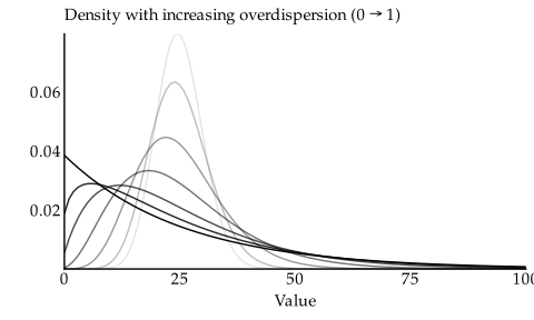
The plot below renders density curves with a \(\mu\) of 25, starting at a transparent Poisson distribution (\(\theta=0\)) and going up to the solid geometric distribution (\(\theta=1\)). If we trace the curves from most transparent to solid, we see how the distribution walks over to the left, merges with the axis (making lower counts more likely), and morphs from Poisson to geometric, all while extreme counts (far to the right) also become larger in magnitude.
In the plot above we stopped at \(\theta=1\), but we could go further into power law territory, and it quickly gets crazy.
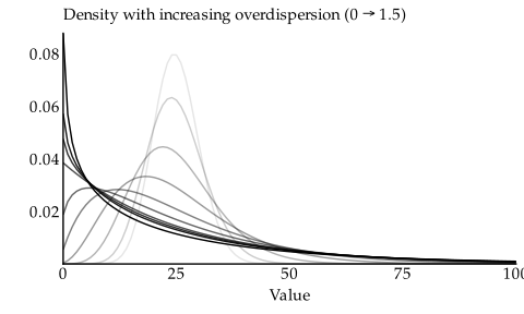
We won’t use this heavy-tailed region in this article, I just wanted to make clear that it doesn’t stop at a \(\theta\) of one – it goes on.
Amazing intuition nobody cares about
Let’s think for a moment about the range between Poisson and geometric, and what happens as we go from one to the other.
Imagine flipping a coin. The geometric distribution models the length of the first uninterrupted sequence of tails. It could be zero if the first toss lands on heads. It would typically be one or two. But it could also be really long, if heads takes its sweet time to show up. In fact, after a sequence of \(n\) tails, the probability of the next tails is still 50/50. This makes the variance of the geometric distribution quite high.
The negative binomial distribution (with \(\theta\) between zero and one) models the total length of multiple sequences of tails. Specifically, it models the length of the first \(r=\frac{1}{\theta}\) sequences of tails. Thus when \(\theta=1\) it models the length of the first sequence, which makes it equivalent to the geometric distribution. When \(\theta=0.5\), it models the combined length of the first two sequences, etc.
To make this make sense, we have to consider what happens to the hypothetical coin as we increase \(r\) (decrease \(\theta\)). We meddle with the probability of the coin so that the expected total number of tails in the sequences stays the same. Thus, when we increase \(r\), we also increase the probability, so that heads are more likely, and thus the length of individual sequences of tails decrease, but their combined length stays the same. Everything else we are going to say works even if we don’t do that, but by keeping the expected total number of tails the same, we can see more clearly how the variance increases, as in the above plots.
When we get into lower \(\theta\) (or higher \(r\)), we are now counting the length of a large number of sequences of tails. The variation in their lengths will sort of cancel out and converge to something more stable. Thus the variance of the negative binomial distribution decreases as we decrease \(\theta\) and make it less overdispersed.
At some point we get to \(\theta \rightarrow 0\), which corresponds to \(r \rightarrow \infty\). At this point, the probability of heads \(p \rightarrow 1\) and we have the Poisson distribution. But note what this means for our interpretation of the Poisson distribution: the events we are counting are the total number of tails in an infinite number of sequences of tails when heads is almost guaranteed to happen on every toss!
Isn’t all this just nuts?5 And what about the heavy-tailed region of the negative binomial distribution? That’s when heads get increasingly rare but we only count a partial sequence of tails to compensate.
Modeling baseball runs as overdispersed counts
Getting back to the problem, we ask our computer to fit a negative binomial distribution to the counts of runs each team scored. It tells us
\[\mu = 4.3,\;\;\;r=3.4\]
We know from the amazing intuition that an \(r\) of 3.4 corresponds to a \(\theta\) of 0.30. It’s difficult to tell from \(\theta\) alone how much overdispersion there is6 We actually get a better idea from the variance which was more than twice the mean. That’s why we started suspecting overdispersion in the first place., but it corresponds roughly to the middle curve on the first plot of increasing \(\theta\). If we try to apply the amazing intuition further, we may think of this as tossing a coin and counting the total number of tails in the first 3.4 sequences of tails, when the coin is only slightly biased toward tails.7 We can tell the bias because \(r \lt \mu\) means the coin is biased toward tails, while \(r \gt \mu\) means the coin is biased toward heads.
I don’t know enough about baseball to translate this into physical processes, but there must be some sort of decision point in the game that happens on average 7.7 times per game, and 44 % of the time when it comes up, it triggers an event that stops the opposing team from scoring a run. When the event has been triggered 3.4 times, the game ends. Note that this doesn’t mean the 3.4th event actually causes the game to end, it means only that the game ends on average after 3.4 such events. Similarly, the lack of an event might not directly cause a run to be scored, it might just be that runs are correlated with the absence of such an event.
Anyway, all of this is irrelevant to forecasting on the question.
Total number of counts for 7 games
We modeled the count for one team in one game as \(\mathrm{NB}(\mu=4.3, r=3.4)\). We want the total number for all seven games in the knockout stages; that’s 14 draws from the distribution above.
Now, the negative binomial distribution has a convenient identity:
\[x_i \sim \mathrm{NB}(r, p) \Longrightarrow \sum_i^n x_i \sim \mathrm{NB}(nr, p)\]
This says that if we have parametrised the negative binomial distribution with \((r, p)\) and we want the distribution of the sum of 14 such random values, we can use the negative binomial distribution with parameters \((14r, p)\).
We don’t have \((r, p)\), though, we have \((\mu, r)\). We could convert that to \((r, p)\) and then convert back, but there’s a more fun way: we can prove a corresponding version of the identity for our parametrisation on our own! We want to find \(\mu'\) and \(r'\) such that
\[x_i \sim \mathrm{NB}(\mu, r) \Longrightarrow \sum_i^n x_i \sim \mathrm{NB}(\mu', r')\]
We start with the parameter transformation
\[p(\mu, r) = \frac{r}{r + \mu}\]
which lets us rephrase the first identity to
\[x_i \sim \mathrm{NB}(r, p(\mu, r)) \Longrightarrow \sum_i^n x_i \sim \mathrm{NB}(nr, p(\mu', nr))\]
For this to be true still, we need to find the value of \(\mu'\) that makes \(p(\mu', nr) = p(\mu, r)\). That means we need to make it so that
\[\frac{r}{r + \mu} = \frac{nr}{nr + \mu'}\]
This happens when \(\mu' = n\mu\) because then we get
\[\frac{nr}{nr + \mu'} = \frac{nr}{nr + n\mu} = \frac{nr}{n(r + \mu)} = \frac{r}{r + \mu}\]
Thus, the identity we are looking for is simply
\[x_i \sim \mathrm{NB}(\mu, r) \Longrightarrow \sum_i^n x_i \sim \mathrm{NB}(n\mu, nr)\]
How convenient.8 The convenience makes it even more strange that I couldn’t find anyone stating this version of the identity. I must have overlooked something.
This means the number of runs scored in the knockout stages of the 2026 wbc is probably distributed as \(\mathrm{NB}(\mu=14 \times 4.3, r=14 \times 3.4)\). That gives us a forecast of 42–80 at 90 % confidence.
The new interval of 42–80 based on more detailed modeling is better (narrower) than the baseline we had at 35–87. That’s what we hoped for. Now that we approached it as the sum of 14 independent-but-lumpy counts, we both used more data to estimate the variation, and we average out some of the noise when we sum it all together.
Go forth and use the negative binomial distribution when appropriate!
Appendix A: On the independence of run counts between teams
In everything above, we treated the run counts from both teams in a game as independent of each other. I could hear an argument that maybe the run counts for the two teams in the same game are not independent. It would make sense for them to be negatively correlated: a good team scores more runs and prevents their opponent from doing the same. That would be bad for us, because that would increase the variation in the count, making our forecast overconfident.
Fortunately, if anything, the correlation appears to be positive. Though it is so weak that fitting the negative binomial model to the number of runs per game rather than per team gives the same forecast interval at 90 % confidence.