The Surprising Richness of Correlations
Traditional wisdom around experimentation says that you should only change one thing at a time, and keep everything else as constant as possible. Fisher, arguably one of the greatest experimentalists of all time, claimed the opposite.
He had a good reason to do so: by systematically varying multiple things simultaneously, we can
- detect effects that would be hidden by confounders,
- attribute effects to their causes more accurately, and
- save money by running one larger experiment instead of many small ones.
And he’s right! I have never been very good at that, though, so I picked up the book where he popularised much of modern statistics.1 Statistical Methods for Research Workers; Fisher; Oliver & Boyd; 1925.
Fisher spends a surprising amount of the book discussing correlations. The way I was taught statistics, the correlation was just a definition to be learned. At best a few pages were spent on it. Almost a quarter of Statistical Methods is about correlations. For context, that’s more than the content on both linear regression and maximum likelihood estimation – together.2 Fisher admits in a later edition that if he were to do the book again, he would reverse this and go for what is today a more traditional approach. I’m glad he didn’t! It’s useful to look at things from multiple perspectives, and I certainly hadn’t seen this correlation-heavy perspective before.
I want to write about the interesting bits on correlation: intraclass correlations and how they tie in to analysis of variance (which is how Fisher made sense of those change-multiple-things-at-a-time experiments). However, before we get there, we need to rehearse the basics of correlations, because I think few people really get them.
Correlations as contributions to variation
We’ll start with data familiar to anyone who meets other people: human heights. It is a common misconception that human heights are normally distributed. We would be forgiven for thinking so too, given the below histogram of human heights.
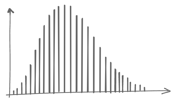
This actually deviates imperceptibly from the normal distribution, because it’s slightly double-peaked: females are shorter than males. We cannot see that when the data is presented this way, because the variation within each sex is large enough to cover up the group-level differences between sexes.
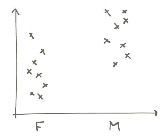
If, on the other hand, we make a scatterplot of sex against height, it becomes obvious even with a tiny sample size:
One way to quantify this difference is by estimating its residual range3 I am now making up terms to get through the example. I don’t think these quantities have real names., which is an indication of how much uncertainty is left once we have accounted for sex. We can imagine the computation this way:
On top of this scatterplot, we draw two pairs of lines.
- One pair of horizontal lines at the top and bottom that capture the full range of all measurements from this sample, and then
- One pair of sloped lines that touch the top and bottom of each of the groups.
We then measure the space between each pair of lines, and we’ll get the following picture.
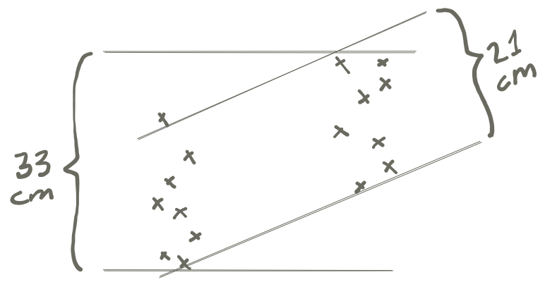
The total range spanned by all of these samples, regardless of group belonging, is 33 cm. The ranges spanned by each of the groups is roughly 21 cm.
What does this give us? Well, if someone asks us to guess the height of any of the people in our sample, it could be any of the tiny crosses, so we’d have to guess a number in a plausible range of 33 cm. However, if we were told the sex that person had reported, we would be guessing only among the crosses on the left or the right, and scare-quote-only have to contend with a plausible range of 21 cm. To quantify how much our guessing range improved, we can divide 21 by 33 and get 0.64, which we will call the residual range left over after controlling for sex. It is the guessing range we have to contend with even when we have accounted for sex, hence the name residual range.
On the flip side, this also gives us a way to quantify how useful the information of reported sex was: we can define accounted-for range to mean the range we accounted for by eliminating variation from sex. This is the inverse of residual range, and since 1−0.64 = 0.36, that latter number is the accounted-for range4 Again, the terms residual range and accounted-for range are entirely my own inventions. These concepts don’t have real names because we have just eyeballed lines on a scatterplot and that’s not what theoretical statisticians do, apparently. of height against sex in our small sample data. In this case, the accounted-for range, i.e. the usefulness of knowing sex, was 0.36.
We can see how a smaller residual range leads to a larger accounted-for range, and this means knowledge of one variable would be more useful for guessing the other.
From accounted-for range to correlation
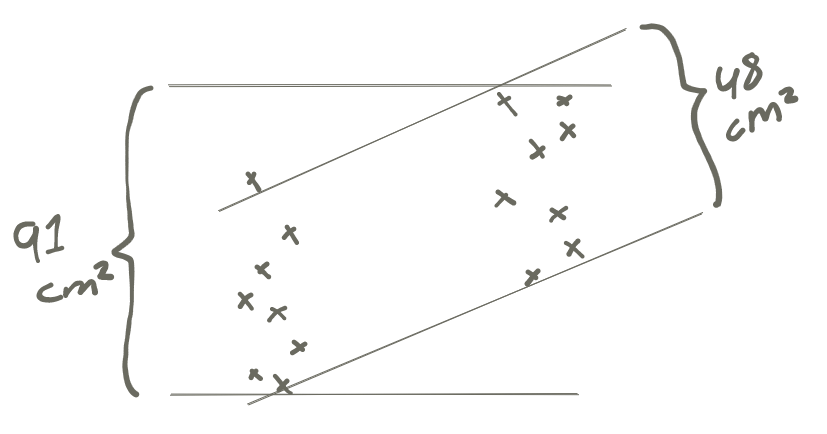
We will make a small change in our procedure for estimating the accounted-for range: Instead of eyeballing the space between the lines on a scatterplot, we will use the variance of the data contained between the lines. With our dataset, the variance of the full data set is 91 cm², whereas the “variance of the sloped lines” – to speak extremely loosely – is roughly 48 cm². This gives us a residual range of 48/91 = 0.53. In turn, this means the accounted-for range is r² = 1−0.53 = 0.47.
When we have used variances (instead of eyeballed ranges) in the computation of the accounted-for range, we can use better terminology. Instead of residual range, we will say coefficient of alienation. Instead of saying accounted-for range, we will say coefficient of determination. These are well-defined quantities, compared to what we got when we eyeballed ranges.
There’s a good reason we use r² as the symbol for the coefficient of determination: its square root is the correlation coefficient. Since in our data r²=0.47, we have r=0.69, and this is indeed the correlation coefficient between sex and height in our data.
We’ll repeat this exact computation again, with visual support, to make it clear: we set the distance between the hypothetical lines based on the variance of (1) the full data set, and (2) the groups individually. Then we get a picture that looks something like this:
The correlation coefficient can be solved out of the equation
\[r^2 = 1 - \frac{\mathrm{variance}(\mathrm{grouped\, data})}{\mathrm{variance}(\mathrm{full\, data})}\]
which in our case was
\[r^2 = 1 - \frac{48}{91}\]
\[r = 0.69\]
This gives an almost-intuitive sense of what this squared correlation coefficient means: it’s the reduction in variance of height from knowing the sex.5 I say almost-intuitive because variances are not intuitive. But they are additive, which is useful as we will see next. Note that from this perspective, the squared correlation coefficient – the coefficient of determination – is a more meaningful number than the correlation coefficient itself.
Correlations from constructing data
We can approach this from the other direction. Let’s imagine we are $deity,
and we do play dice with the universe. The mission for today is creating a
human. For our purposes, this is a two-step process: first we randomly select a
sex, and then we randomly assign some genetic variation in height from there.
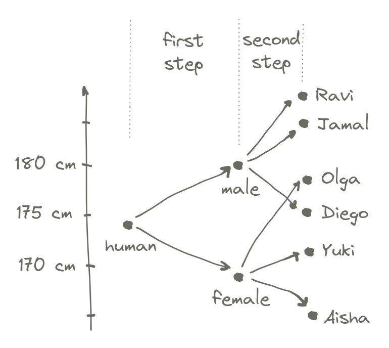
We start with the average height of all humans, which is something like 174 cm. Then we toss a coin to see which sex it will be. if it’s male, we set a baseline height that is 6 cm over the human average, and if it’s female, we set the baseline 7 cm under the average.6 These particular numbers might not make all that much sense. This is because they are derived from the small sample above, to make the results line up nicely. Then we throw one of those normally distributed dice to select genetic contributions on top of that. Tadaa! A fully formed individual.
The total variance in height produced by this entire process is somewhere around 91 cm². This should not come as a surprise, as we had already established that the total variance of our full data set was 91 cm². A great thing about variances from independent sources is that they are additive. Since there are two (independent) steps in creating a human, we know we have an equation of the form
\[\mathrm{variance}(\mathrm{first\,step}) + \mathrm{variance}(\mathrm{second\, step}) = 91\]
If we compute the variance of the first step (a coin toss with −7 or +6 as the outcome) we will learn it is roughly 41 cm². Solving the full equation, we get
\[41 + 48 = 91\]
Hey, doesn’t that other term look familiar? Sure enough, we have
\[r^2 = \frac{41}{91}\]
This is another lens through which we can intuit the squared correlation coefficient. If we construct a random variable first through a group-level effect, and then add individual variation on top of that, the squared correlation between the variable and the group is exactly equal to the variance of the group-level effect divided by the total variance.
Phased differently, in a multi-step process, the correlation between the nth variable and the end result is the fraction of the total variance contributed by the nth step.
Quick and dirty significance of correlations
There is a good way to figure out whether a correlation is significant or not, but there is also a quick and dirty way. The reason it’s dirty is it makes plenty of assumptions that break down fairly easily in real life situations, including when,
- The sample size is small,
- The correlation is close to ±1, or
- The correlation is close to 0.
In other words, it breaks down very frequently. But we’ll learn it anyway for a quick back-of-the-napkin estimation of significance. It gives the standard error of the correlation coefficient \(r\) as approximately
\[\mathrm{se}_{r} = \frac{1 - r^2}{\sqrt{n-1}}.\]
The reason this is useful to learn is it only requires us to roughly estimate the coefficient of determination and the sample size to get quick experiment power calculations.7 Imagine we have a phenomenon which we think is mainly caused by four things. This means each thing might contribute something like 20 % of the variance. If we can afford a sample size of 200, is it worth bothering with the experiment at all? It turns out yes, it might be. We can approximate the standard error as \(0.8/16 \approx 0.05\), which is enough to detect the effect if it exists with the presumed correlation. The reason this works is that all statistical tests in common use (even those that don’t mention correlations!) are effectively equivalent to a correlation significance check.8 If a linear regression coefficient is significant, then also its correlation with the outcome will be significant, and vice versa. If a \(z\) test is significant, then the corresponding correlation coefficient will also be significant, and so on.
As a concrete example, for the correlation \(r=0.69\) for the height data above, which was taken from 16 measurements, we compute the standard error
\[\frac{1 - 0.69^2}{\sqrt{15}} \approx 0.14\]
Since the correlation, 0.69, is over five times larger than 0.14, we can probably hopefully think of this result as significant, even though we likely violated the large-sample assumption of this computation.
To reiterate: this approximation of the standard error is really only dividing what we called the residual range by the square root of the number of observations. It’s saying that if the residual range is large, we are more likely to accidentally get spurious correlations through sampling error – exactly what a significance check should do.
Moving to fully continuous data on both axes
In the previous example, we had dichotomous data on the x-axis. This is a particularly convenient situation because we can easily intuit the data as belonging to either one group or the other. But to use correlations to their potential, we need them to apply to fully continuous data. Fortunately, this is a relatively straightforward extension of what we have already seen.
Measuring the correlation between room count and income
I have sampled 18 people living in my area of town9 Which is a fairly homogeneous area, making it harder to get strong correlations, unfortunately., and compared their income to how many rooms there are in their domicile.10 Since the data depends on income, I sadly had to exclude people with female-sounding names to avoid having gender-based income differences masking the effect we’re looking for. It’s hard to pretend these differences don’t exist when one has spent even a few seconds looking at the data. Here is the scatterplot that came out of that.
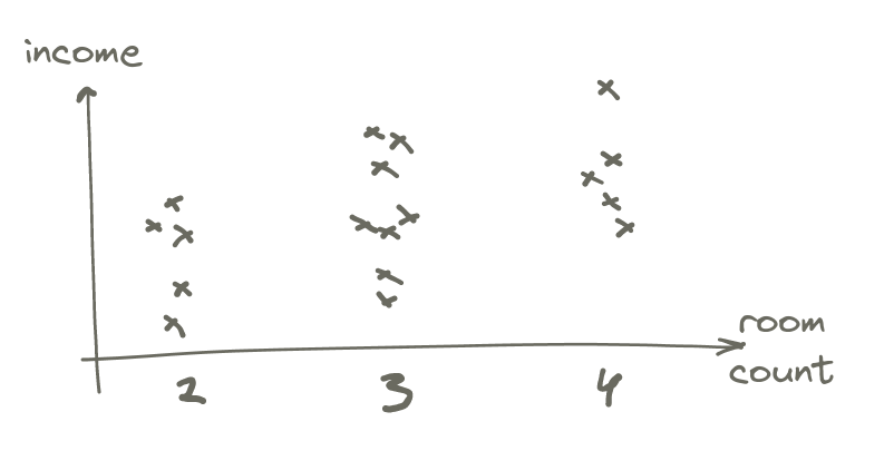
It’s clear the number of rooms increase with income, but there’s also a large overlap, so we would expect the correlation to be positive, but at the lower end – and it is: 0.34.11 The quick and dirty standard error is 0.21, making this 1.6 standard errors away from zero – very close to the fast and loose threshold of 1.645 I often use informally to determine if I should investigate further.
If we think of this as a two-step generation process, we can imagine that the variance we introduce by first assigning a baseline income as the average given that room count is about a ninth of the total variance of income.12 Remember that since r=0.34 we have r²=0.12 – and this is the variance due to room count, with the rest being due to other factors. Most of the variance comes from individual factors beyond that.
This example works just the same as before, except there are three levels possible for the group assignment rather than two.
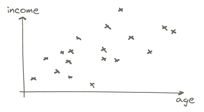
Correlation between age and income
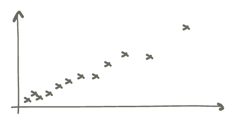
We can continue extrapolating from two to three levels, and then to an infinite number of levels, when the x axis is on a continuous scale instead. Here is income against age.
When taking the correlation between two continuous variables, we are still doing the same thing as before: drawing lines that capture the variance of the total data, and then of the conditional distribution13 Since variance is based on squared deviation, when applied to income it has units of dollars squared.:
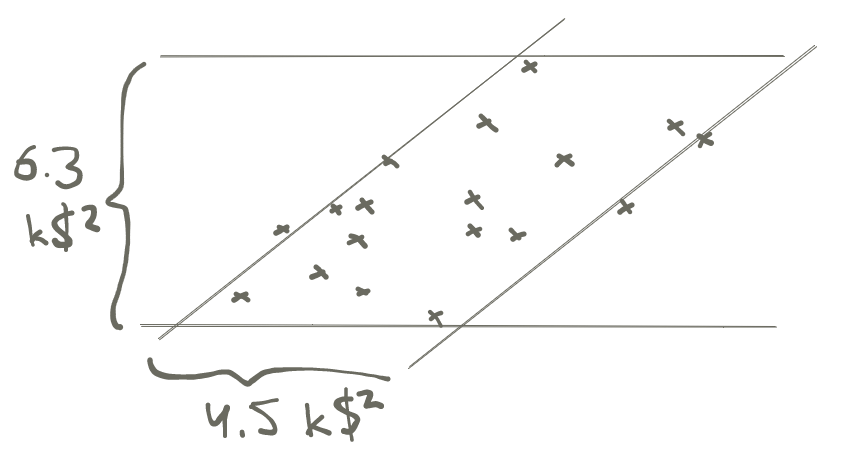
These variances imply a correlation of
\[r = \sqrt{1 - \frac{4.5}{6.3}} = 0.53\]
which is indeed the correlation between age and income in this data. The interpretation of this, going back to the lines above, is that about 2/3 of the variance of the income distribution is independent of age.14 To be clear, I selected for inclusion in the data only people that appeared to be working. If we include retirees, the age-vs-income curve looks like an arch, with income increasing until retirement age, then decreasing again.
We can still sort of think of this as first assigning people to an age with a corresponding mean income for that age, and then applying individual factors on top of that. The correlation says that only 1/3 of the variance in income will come from the differences between the means for each age.15 And here we might have a candidate for further consideration: the correlation is 3 standard errors away from zero.
Correlation between correlations, partial correlations
For the email updates from this site, I include an estimated reading time when referencing new articles.
At first I computed this by looking up a slow and fast reading speed, counting
words in the source file with wc and performing the computation. Then I
thought maybe I can pipe the published article into the llm cli and ask
Claude 3.5 Sonnet for a word count. On the article I tried, it nailed it very
closely. I got curious: was that a fluke or is it consistent?
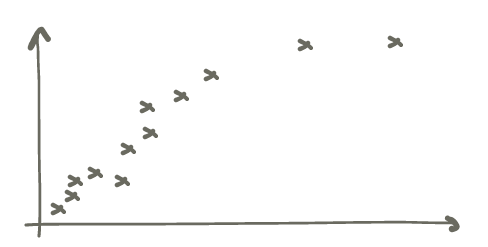
On the x axis we have word count by wc, and on the y axis by Claude. Claude
consistently underestimates the word count compared to wc, but it is
possible Claude tries to ignore sidenotes, metadata, and certainly does not see
the code that’s in the source file but never exported, so this is expected.
This is remarkable! The correlation is 0.98. It does get some articles very wrong (one 6700-word article has 4500 words according to Claude, even after adjusting for the persistent underestimation) but on the whole, it has the right idea for what a word count is, at least.
By the way, are you not yet a subscriber to email updates? You might like it better than rss because there are article summaries and bonus content. And I promise to be responsible with your inbox. See subscription options and archives of past emails. If you don't like it, you can unsubscribe any time.
Proper significance test through z conversion
Since this correlation is close to ±1, and from a small sample to boot, we should not use the quick and dirty significance estimation.16 It would suggest the correlation is 84 standard deviations away! What we do instead is convert the correlation to a \(z_r\) value through this function:
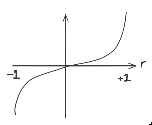
This function captures the intuition that a difference in correlation coefficient between, say, 0.9 and 0.95 is much more significant than that between 0.2 and 0.5
Formally, the conversion is
\[z_r = 0.5 \log{\frac{1+r}{1-r}}\]
The standard error of \(z_r\) does not, remarkably, depend on \(r\) at all, but is given plainly by
\[\mathrm{se}_{z_r} = \frac{1}{\sqrt{n - 3}}\]
We find in this case that we have \(z_r =\) 2.3, with a standard error of 0.33, which means the correlation is seven standard errors away – much more reasonable than the naïve approximation.
Second correlation in almost the same data
We can perform the same exercise with gpt-4, another popular high-end model these days. It looks closer to this:
The correlation here is 0.93 – still very high, but not as impressive.
Partial correlation, controlling for other variables
We might be interested in finding out whether the counts by Claude and gpt-4 are correlated. This would imply they tend to make mistakes in the same direction when asked to count words in the same articles. That would be interesting! Since they are developed completely independently, if they generally make mistakes in the same direction, that is evidence in favour of those mistakes being embedded in their architecture, rather than the specifics of their training.
The correlation between the count by Claude and gpt-4 is 0.91. At first glance, we might take this to mean that they do indeed make mistakes in the same direction. But on closer thought, that’s not at all what we are measuring with that correlation. We knew both are decent at predicting the true word count, so clearly their counts will be strongly correlated – because they are strongly correlated with the true word count!
If anything, the fact that the correlation between the counts by Claude and gpt-4 is lower than the correlation between either and the true word count might suggest that their counts are negatively correlated, i.e. that they make mistakes in opposite directions. We’ll see.
We need to somehow compute a correlation between the counts by Claude and
gpt-4 that controls for the true word count. We can, in fact, do this. Fisher
calls this a partial correlation and we could write it as \(r_{cg,w}\),
indicating that we are looking for the partial correlation betwwen Claude and
gpt, controlling for the word count as reported by wc.
To compute \(r_{cg,w}\), we need the three correlation coefficients for the three pairs of variables: \(r_{cg}\), \(r_{wg}\), and \(r_{wc}\). We have those! Then the formula is
\[r_{cg,w} = \frac{r_{cg} - r_{wg} r_{wc}}{\sqrt{(1-r_{wg}^2) (1 - r_{wc}^2)}}\]
In our case, we’ll evaluate this as
\[r_{cg,w} = \frac{0.91 - 0.93 0.98}{\sqrt{(1-0.93^2) (1 - 0.98^2)}} \approx -0.26\]
Indeed! Our intuition was correct: the counts by Claude and gpt-4 are somewhat negatively correlated, indicating they make mistakes in opposite directions. That would be just as surprising as them making mistakes in the same direction. Fortunately, this result is not significant. Both the quick and dirty approximation and the more thorough computation based on \(z_r\) indicate this correlation is just under one standard error from zero.17 Note that when computing a partial correlation, we are removing one digree of freedom, which means for significance computations we must use \(n-1\) instead of \(n\) everywhere. For each variable controlled for, there is one degree of freedom removed.
Next stop: intraclass correlation
One of the questions we asked above is
What is the correlation between income and room count?
There is a very similar question we could ask instead, namely
What is the correlation in income between pairs of people who have the same room count?
It turns out these two questions have the same numerical answer. Both measure the correlation between income and room count. But! By phrasing it in terms of pairs of subjects that share a property, we can compute correlations that would otherwise be difficult. For example
What’s the correlation between commit size and programming language?
is an interesting question, but it’s difficult to imagine how we can scatterplot that. Commit size would be on the Y axis, but it’s unclear what to do on the X axis18 If we had just two programming languages, we could do what we did with the height–sex correlation and put the two programming languages as two groups on the X axis because at that point order doesn’t matter for the result. But there are more than two programming languages!, because “programming language” is a nominal scale, not an ordinal one. However, if we rephrase the question in the way we just learned,
What’s the correlation in commit size between pairs of commits on source files using the same programming language?
we can totally plot that! Now we have commit size on both X and Y axes, and the marks on the plot correspond to pairs of commits to source files in the same programming language.
This leads us into what is known as intraclass correlation, and then further into anova. These are things that may end up being a separate article, because this one is long enough already. I hope you enjoyed learning this as much as I did!